Fundamentals of Statistics

Sir Arthur Lyon Bowley

Statistics:

In the simplest form, Statistics is defined as a numerical representation of information. According to a renowned English statistician Sir Arthur Lyon Bowley, statistics refers to numerical statements of facts in any area of inquiry.

Sir Arthur Lyon Bowley, also an economist, worked on economic statistics and pioneered the use of sampling techniques in social surveys.

Statistics is also seen a branch of mathematics which deals with enumeration data (one type of numerical data). Statistics is used as a tool in data analysis of a research; it is used to gather, organize, analyze, and interpret information gathered.

Let’s first understand what the data is. Data refers to a set or a bundle of information which is collected in order to conduct a research. Data is of two types: Numerical, and Non-numerical.

The data that can be counted is termed as numerical data; it deals with numbers and calculation, whereas non-numerical data deals with information which cannot be counted rather it is inferred or assumed.

Though both types of data (numerical as well as non-numerical) are information, the role of statistics is confined to “numerical data” only.

Numerical data is of two types—enumeration data, and metric data. Enumeration data refers to information which can be counted, for example, class intervals, frequencies, etc. Metric data is based on measurement; it needs unit specification in order to make sense of data.

Branch of Statistics:

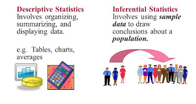
There are two major branches of statistics—“Descriptive Statistics”, and “Inferential Statistics”.

Descriptive Statistics: 

It describes certain characteristics of a group of data. It has to be precise (precise means brief and exact). It limits generalization to the particular group of individuals observed. Hence, no conclusions are extended beyond this group, and any similarity to those outside the group cannot be assumed. The data describe one group and that group only.

Inferential Statistics: 

It is related to the estimation or prediction based on certain evidence. It always involves the process of sampling and the selection of a small group. This small group is assumed to be related to the population from which it has been taken. The small group is known as the sample, and the large group is the population. Inferential Statistics allows the research to draw conclusions about populations based on observations of samples.

Following are the two important goals of inferential statistics:

·         The first goal is to determine what might be happening in a population based on a sample of the population.

·         And the second goal is to determine what might happen in future.

Thus, inferential statistics are to estimate and/or to predict. In order to use inferential statistics, only a sample of the population is required.

Organization of Data:

Ordered Array: 

It refers to the data (a set of information) which is arranged in descending order, for example, 90, 80, 75, 68, 60. The Ordered Array, also known as Set, provides a more convenient arrangement. The highest score is 90 and lowest score is 60 are easily identified. In this way, the range (the difference between the highest and the lowest scores, plus one) can be easily determined.

Grouped Data: 

The data which can be presented in the form of class interval and frequency is known as the Grouped Data. In this way of presentation, the data are often more clearly presented. Data can be presented in frequency table with different class intervals, depending on the number and range of the scores. There is no rule that rigidly determines the proper score interval. However, intervals of 10 are frequently used. 

Read More

What are Measures of Variability?

Measures of variability are also called the measures of spread or dispersion. It lets the researcher know how scattered the scores are from their central tendency.

For example, if a group is homogeneous (containing individuals of nearly the same ability), most of its scores will fall around the same point on the scale; therefore, the range will be relatively short and the variability will be small.

But, if the group is heterogeneous (having individuals of widely differing capacities), scores will be strung out from high to low; thus, the range will be relatively wide and the variability will be large.

In order to indicate the variability or dispersion, the following four measures have been devised. These are:

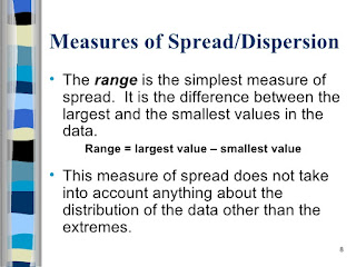
1.    Range: It is the simplest form of measures of variability. It is the difference between the highest and the lowest scores in a distribution. Range is the crudest form of variability as it considers the extremes scores only. It is not a stable statistic (unreliable) because its value can differ from sample to sample drawn from the same population.

2.    Quartile Deviation: The quartile deviation (generally represented by “Q”) is one-half of the scale distance between the third quartile (75^th percentile) and the first quartile (25^th percentile) in a frequency distribution. First quartile is a point below which 25 percent of the scores lie, while the third quartile refers to the point below which 75 percent of the scores lie. Quartile Deviation (QD) is preferred when scores are widely dispersed or scattered.

3.  Average Deviation: It is also called “Mean Deviation”. It refers to the average of deviation of all scores from their mean. It does not consider signs (negative and positive) of the scores; that is, all deviation whether plus or minus are treated as positive.

4.     Standard Deviation: Standard Deviation (SD) is the square root of variance. It is the most stable form of measures of variability. It is employed in experimental work. Variance refers to the average of the square deviations of the measures or scores from their mean. Standard Deviation (SD) is used when scores are not widely dispersed or scattered.

Read More

What are Parametric Tests & Non-Parametric Tests?

Parametric Tests & Non-Parametric Tests

Parametric Tests (for example, “t” test, and “f” test) are regarded as one of the most powerful tests. It is used during the stage of data analysis of a research work.

Parametric Tests are used when certain basic assumptions are fulfilled. If those assumptions are not fulfilled, that kind of tests comes under the ambit of Non-Parametric Tests (such as, chi square test, and Mann-Whitney Test).

Following are the basic assumptions of the parametric tests. If these assumptions are fulfilled, then parametric tests could be used; otherwise, non-parametric tests would be employed. Let’s discuss the basic assumptions of:

1.    Normality of Distribution: The sample (which has been drawn from the population) must be normally distributed for parametric tests. If samples are not normally distributed, it would not fall under the category of non-parametric tests; that is why, non-parametric tests are also known as distribution-free tests.

2. Randomization: The condition for selecting sample from the populations must be random. It means any technique, which is under the category of probability sampling technique, needs to be adopted. If samples are not selected through the process of randomization, we cannot apply parametric tests; in that case, we would apply non-parametric tests.

3. Homogeneity of Variance: The samples have equal, or nearly equal, variances. Homogeneity means sameness (in other words, more or less it should be same). For example, if we calculate the variance of two populations from where samples are drawn, they must have more or less same variance.  If there is a wide difference among the variance of the sample, parametric tests cannot be used; in such case, non-parametric tests will be used.

4.   Null-Hypothesis: This assumption is pre-requisite for both parametric as well as non-parametric tests. Therefore, this assumption is not the distinctive feature of parametric tests; this is the common feature of both parametric and non-parametric tests.

In both type of tests (parametric test or non-parametric test), a null-hypothesis must be formed. A null-hypothesis states that there is no significant difference or relationship between two or more parameters.

What are Parametric and Non-Parametric Data?

There are two types of data which are recognized during the application of statistical treatments. These are the following:

        i. Parametric Data: It refers to the data which are measured. As it has already been discussed above, parametric tests assume that the data are normally (or nearly normally) distributed. Parametric tests are applied to both interval and ratio scaled data.

     ii.Non-Parametric Data: Data of this type are either counted (nominal) or ranked (ordinal). 

Read More

Measures of Central Tendency

Mean, Median, Mode and Range

When scores are tabulated into a frequency distribution, calculation of measures of central tendency (or central position) follows. Measures of central tendency can be better understood this way, for example, if we compress the entire distribution at one single point, then that single point represents the central tendency. Measures of central tendency are sometimes called measures of central location.

Score is the measurement of individual performance by means of tests. And when scores are expressed in equal units, they form an interval scale.

The value of a measure of central tendency serves two purposes. First, it is an “average” which represents all the scores. Second, it enables the researcher to compare two or more groups in terms of typical performance.

There are three “averages’ or “measures of central tendency” which are in common use. These are: (1) Mean, (2) Median, and (3) Mode.

Mean: It is an “arithmetic” mean. Mean is probably the most familiar average. The mean (of a set of scores) is the sum of separate scores (or measures) divided by their number.  It is used to describe the middle of a set of data.

Advantage of Mean:

1. Most popular measure. 

2. It is unique, there is only one answer.

Disadvantage of Mean:

1. It is affected by extreme values/scores.

Median: It is a “positional” average. When ungrouped scores (also known as raw data) are arranged in order of size, the median is the midpoint in the series. It is a measure of position rather than of magnitude.

Advantage of Median:

Extreme values do not affect the median as strongly as they affect the mean.

Disadvantage of Median:

It takes relatively long time to calculate for a very large set of data.

Mode: It is a “democratic” average. It is defined as the most frequently occurring score in a distribution. If there is only one value which occurs a maximum number of times, then the distribution is said to have one mode.

Advantage of Mode:

1. It is easy to understand and simple to calculate.

2. It is not affected by extreme large or small values.

3. It can be useful for qualitative data.

Disadvantage of Mode:

1. It is not used more frequently as compared to mean and median.

2. It is not necessarily unique; there may be more than one answer.

3. When no values repeat in the data set, the mode is every value and is useless.

4. When there is more than one mode, it is difficult to interpret and compare.

Read More